Using INDEX MATCH in Google Sheets

Can you use INDEX MATCH in Google Sheets?

INDEX MATCH in Google Sheets can be used as a combination of the 2 functions INDEX and MATCH. Using these two formulas allows you to pinpoint and extract data from an array with precision, revolutionizing the way you work with your spreadsheets. Unlike traditional methods, this dynamic duo adapts to changes in your data, making it a versatile solution for various scenarios.

‍

How to use the INDEX function in Google Sheets

Let’s start from the basics. The INDEX function is very basic itself. It returns the value of a specific cell based on its row and column numbers. Nothing too fancy. Its syntax is as follows:

INDEX(reference, [row], [column])

Where:

reference is the array of data your cell is in (headers excluded)

Row is the rows number within the array where the cell is

Column is the column number within the array, where the cell is.

In this example, to return the value of Jim Halbert salary we will use the following syntax: =INDEX(B9:E21,4,3)

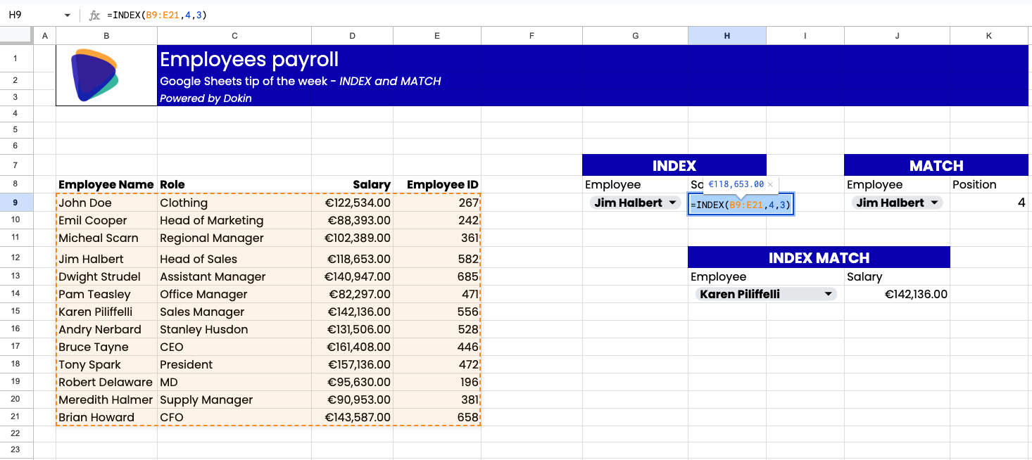
That returns the value of Jim Halbert salary, but as you can see, it is a pretty pointless function on its own, as it is pretty manual and doesn’t allows us to return the value for a different set of keys.That’s when the MATCH function comes to the rescue.

‍

How to use the MATCH function in Google Sheets

The MATCH function returns the position of a specific key within a range of data. Its syntax is as follows:

MATCH(search_key, range, [search_type])

Where:

Search_key: is the value to search for

Range: The one-dimensional array to be searched for that value

Search_type: determines an approximate or exact match. (enter 0 for exact match).

In the following example, the syntax =MATCH(J9,B9:B21,0) returns the position of the value “Jim Halbert” within the Employee name array.

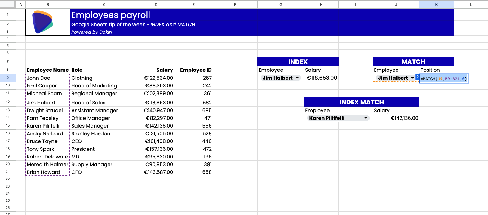
Jim Halbert is in position number 4 within the array selected.

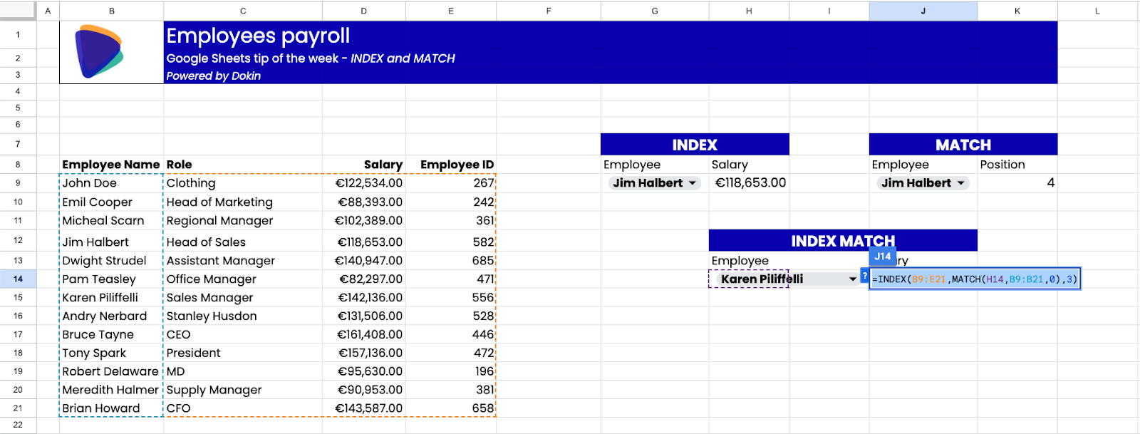
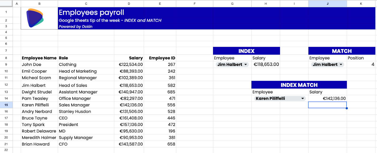
This means that if we combine INDEX and MATCH we can return the value of each employee automatically when it is entered in the selector.

Let’s see how.

‍

How to use INDEX MATCH in Google SheetsI

INDEX and MATCH combined together, allow you to return the value of a cell of an array based on the position of a defined argument. The syntax in the following example, allows us to return the salary of the employee selected in cell H14:

=INDEX(B9:E21,MATCH(H14,B9:B21,0),3)

‍

‍

VLOOKUP vs INDEX MATCH in Google Sheets

(checkout our complete guide on VLOOKUPS and XLOOKUPS)

VLOOKUP and INDEX MATCH have a common purpose, which is returning a specific value in an array based on an argument. It is hard to define a “superior solution” as it ultimately comes down to personal taste, choices and also sets of data you are working with. I personally am a great user of LOOKUPs, particularly XLOOKUPs lately, but I prefer to use INDEXMATCH when I am working on large datasets in spreadsheets shared with many users, as it makes formulas more rigid and reliable and gives me a sense of additional comfort in terms of security of data when I know that others may be using my tables. Overall, though, there is not a clear winner, it comes down to your own preference and comfort.

‍

How do I INDEXMATCH between Sheets?

Using INDEXMATCH between different Sheets is pretty simple. After delcaring the INDEX or the MATCH function, you need to declare the array arguments. To do that, simply select the array you need to retrieve data from, even by browsing onto a different sheets. In this way, you'll be able to INDEX and MATCH the data across different tabs of a spreadsheets or even different Sheets.

‍

Conclusion

Combining the INDEX and MATCH functions allows you to return data from a specific array based on a matching key. It is a powerful combination that offers a solid alternative to XLOOKUPS and VLOOKUPS and can be particularly useful when you are managing large datasets. Use it particularly in those cases where you share sèreadsheets made of large datasets with other users, to ensure that data lookups are hurdled in specific sets of criteria.